Cloudy SolarSoftware: Difference between revisions
imported>Elaszlo No edit summary |
imported>Elaszlo No edit summary |
||
| Line 16: | Line 16: | ||
== Introduction == | == Introduction == | ||
In our project "Extending the Virtual Solar Observatory ([http://umbra.nascom.nasa.gov/vso/ VSO])," we have combined features available in Solar Software ([http://hesperia.gsfc.nasa.gov/rhessidatacenter/software.html SSW]) to produce an integrated environment, supporting data location, retrieval, preparation, and analysis. This workflow in shown Figure 1 with examples given below. Our goal is an integrated analysis experience in IDL, easy-to-use but flexible enough to allow more sophisticated procedures such as multi-instrument analysis. To that end, we have made the transition from a locally oriented setting where all the analysis is done on the user’s computer, to an extended analysis environment where IDL has access to services available on on other computers through the Internet. We have implemented a form of [http://en.wikipedia.org/wiki/Cloud_computing Cloud Computing] that uses the VSO search and a new data retrieval and pre-processing server ([https://team.i4ds.ch/projects/JIDL PrepServer]) that provides remote execution of instrument-specific data preparation. The raw and pre-processed data can be displayed with our GUI plotting suite, [http://hesperia.gsfc.nasa.gov/ssw/gen/idl/plotman/doc/plotman_help.htm PLOTMAN], which can display different data types and perform basic data operations. | In our project "Extending the Virtual Solar Observatory ([http://umbra.nascom.nasa.gov/vso/ VSO])," we have combined features available in Solar Software ([http://hesperia.gsfc.nasa.gov/rhessidatacenter/software.html SSW]) to produce an integrated environment, supporting data location, retrieval, preparation, and analysis. This workflow in shown Figure 1 with examples given below. Our goal is an integrated analysis experience in IDL, easy-to-use but flexible enough to allow more sophisticated procedures such as multi-instrument analysis. To that end, we have made the transition from a locally oriented setting where all the analysis is done on the user’s computer, to an extended analysis environment where IDL has access to services available on on other computers through the Internet. We have implemented a form of [http://en.wikipedia.org/wiki/Cloud_computing Cloud Computing] that uses the VSO search and a new data retrieval and pre-processing server ([https://team.i4ds.ch/projects/JIDL PrepServer]) that provides remote execution of instrument-specific data preparation. The raw and pre-processed data can be displayed with our GUI plotting suite, [http://hesperia.gsfc.nasa.gov/ssw/gen/idl/plotman/doc/plotman_help.htm PLOTMAN], which can display different data types and perform basic data operations. Figures 1, 2, and 3 show the entire framework with numbers corresponding to steps 1-2-3 explained below in the text. | ||
Our environment supports data from a growing number of solar instruments that currently includes RHESSI, SOHO/EIT, TRACE, SECCHI/EUVI, HINODE/XRT, and HINODE/EIS. | Our environment supports data from a growing number of solar instruments that currently includes RHESSI, SOHO/EIT, TRACE, SECCHI/EUVI, HINODE/XRT, and HINODE/EIS. | ||
<gallery caption="Overview of the Cloudy SolarSoftware concept" perrow="3"> | |||
Image:CloudySSW.Step1.png|'''Figure 1.''' SHOW_SYNOP allows searching the VSO from within SSW IDL for solar data (Step 1). | |||
Image:CloudySSW.Step2.png|'''Figure 2.''' Data found with SHOW_SYNOP can be sent to the PrepServer for pre-processing (Step 2). | |||
Image:CloudySSW.Step3.png|'''Figure 3.''' This figure shows examples of image data displayed with PLOTMAN. The images in the first two columns show pre-processed images. The third column shows the images in column one overlaid as contours on the images in column two (Step 3). | |||
</gallery> | |||
== Minimum Requirements == | == Minimum Requirements == | ||
| Line 29: | Line 35: | ||
=== Step 1: Finding the Data === | === Step 1: Finding the Data === | ||
[http://hesperia.gsfc.nasa.gov/~zarro/synop/show_synop.html SHOW_SYNOP] shown in Figure | [http://hesperia.gsfc.nasa.gov/~zarro/synop/show_synop.html SHOW_SYNOP] shown in Figure 4 is an IDL graphical user interface (GUI) to search for and retrieve instrument data within a specified time interval using the VSO or other data finding facilities. | ||
Search results can be directly downloaded into the active SSW IDL environment. To start searching with SHOW_SYNOP, first open the GUI by typing <code>SHOW_SYNOP</code> in your SSW IDL environment command-line. The red box highlights the VSO search form with "Start Time" and "End Time" specifying the search interval and "remote sites ->" defining the instrument (TRACE in this example). Click on the "Search" button to query the VSO for data files that will be displayed in the list below the search form shown in the green box. | Search results can be directly downloaded into the active SSW IDL environment. To start searching with SHOW_SYNOP, first open the GUI by typing <code>SHOW_SYNOP</code> in your SSW IDL environment command-line. The red box highlights the VSO search form with "Start Time" and "End Time" specifying the search interval and "remote sites ->" defining the instrument (TRACE in this example). Click on the "Search" button to query the VSO for data files that will be displayed in the list below the search form shown in the green box in Figure 5. | ||
For information on command-line VSO data searching, please click [[#Step_1:_Finding_the_Data_2|here]] | For information on command-line VSO data searching, please click [[#Step_1:_Finding_the_Data_2|here]] | ||
<gallery caption="SHOW_SYNOP for finding data" perrow="2"> | |||
Image:CloudySSW.Show_synop.Search.png|'''Figure 4.''' This is a screen shot of the SHOW_SYNOP GUI used to find and retrieve specific data sets within a given time interval. The red box indicates the VSO search form (start/ent time and instrument). This screen shot also shows the extensive list of instruments available for search. | |||
Image:CloudySSW.Show_Synop.Searched.png|'''Figure 5.''' The green box marks the result list window in SHOW_SYNOP, and the yellow-framed button opens the configuration menu. | |||
</gallery> | |||
=== Step 2: Pre-processing === | === Step 2: Pre-processing === | ||
Typically, instrument data found with the VSO are unprocessed level-0 data. The PrepServer offers remote pre-processing of those data from within SHOW_SYNOP or from the IDL command-line before or after downloading. In SHOW_SYNOP, search results are displayed in the list underneath the VSO search form (see Figure | Typically, instrument data found with the VSO are unprocessed level-0 data. The PrepServer offers remote pre-processing of those data from within SHOW_SYNOP or from the IDL command-line before or after downloading. In SHOW_SYNOP, search results are displayed in the list underneath the VSO search form (see Figure 5, green box). There are two different pre-processing behaviors configurable: | ||
* By default a click on "Download" retrieves the level-0 data file, stores it on the local hard drive and adds it to a list (Figure | * By default a click on "Download" retrieves the level-0 data file, stores it on the local hard drive and adds it to a list (Figure 6, blue box). The level-0 data file is pre-processed by selecting it in the blue box and clicking on "Display". This uploads the level-0 data file to the PrepServer where it is pre-processed, and downloads the pre-processed product to the local hard drive. | ||
* In auto-preprocessing mode, which can be activated in the configuration menu ( | * In auto-preprocessing mode, which can be activated in the configuration menu (Figures 5 and 7, yellow box), SHOW_SYNOP sends the URL of the level-0 data file to the PrepServer and only downloads the pre-processed data. | ||
In case of zipped data files (e.g. TRACE), SHOW_SYNOP opens a selection widget to help choosing the desired image(s) (see Figure 8). | |||
<span style="color:#FF0000">Please note: SHOW_SYNOP and the PrepServer are dependent on data providers for downloading speed. Be aware that downloading data may take a few minutes, during which SHOW_SYNOP or your SSW IDL session may be unresponsive.</span> | <span style="color:#FF0000">Please note: SHOW_SYNOP and the PrepServer are dependent on data providers for downloading speed. Be aware that downloading data may take a few minutes, during which SHOW_SYNOP or your SSW IDL session may be unresponsive.</span> | ||
For information on command-line data pre-processing, please click [[#Step_2:_Pre-processing_2|here]] | For information on command-line data pre-processing, please click [[#Step_2:_Pre-processing_2|here]] | ||
<gallery caption="SHOW_SYNOP for downloading and pre-processing data" perrow="3"> | |||
Image:CloudySSW.Show_synop.Downloaded.png|'''Figure 6.''' In this screen shot of SHOW_SYNOP the window highlighted in blue indicates the local file repository with level-0 and pre-processed data files. | |||
Image:CloudySSW.Show synop.Options.png|'''Figure 7.''' This options menu allows configuring the pre-processing behavior: download level-0 data or request pre-processed data. | |||
Image:CloudySSW. | Image:CloudySSW.Selection.Widget.Figure4.png|'''Figure 8.''' When pre-processing a TRACE data file that contains multiple TRACE images, a selection widget will open allowing picking a set of images. | ||
Image:CloudySSW. | |||
Image:CloudySSW. | |||
</gallery> | </gallery> | ||
=== Step 3: Visualizing === | === Step 3: Visualizing === | ||
The data are visualized with PLOTMAN, which handles different data types such as light curves, images, spectra, and spectrograms. It provides basic display operations such as zooming, image overlays, solar rotation, etc. To display data with PLOTMAN from within SHOW_SYNOP, simply select a data file (Figure | The data are visualized with PLOTMAN, which handles different data types such as light curves, images, spectra, and spectrograms. It provides basic display operations such as zooming, image overlays, solar rotation, etc. To display data with PLOTMAN from within SHOW_SYNOP, simply select a data file (Figure 6, blue box) and click on "Display". If the data file has already been pre-processed, it will be displayed immediately in a PLOTMAN window. Otherwise, it is first sent to the PrepServer for processing. If multiple files have been selected, all are displayed in the same PLOTMAN window (see Figures 9, 10, and 11). | ||
Like all other GUIs discussed in this nugget, PLOTMAN can also be called from the command-line. Examples can be found [[#Step_3:_Visualizing_2|here]]. | |||
<gallery caption="Example images displayed with PLOTMAN" perrow="3"> | |||
Image:CloudySSW.XRT.Figure3.png|'''Figure 9.''' This figure shows PLOTMAN displaying an XRT image (January 25 2007 06:56:56) that has been pre-processed with default settings by the PrepServer | |||
Image:CloudySSW.TRACE.Figure5.png|'''Figure 10.''' This figure shows PLOTMAN displaying a TRACE image (171 A, January 25 2007, 06:15:09) that has been pre-processed with default settings by the PrepServer. If multiple images were selected in the selection window (see Figure 8), they can be accessed by clicking on "Window_Control" in PLOTMAN's menu panel at the top. | |||
Image:CloudySSW.RHESSI.EIT.Overlay.Figure.6.png|'''Figure 11.''' This figure shows PLOTMAN displaying an contour overlay of a reconstructed RHESSI clean 6-12keV image on an EIT image (171 A, January 25 2007, 07:00:13). The reconstruction of the RHESSI image as well as the pre-processing of the EIT images was done with the PrepServer. | |||
</gallery> | |||
== IDL Command-Line Tools == | == IDL Command-Line Tools == | ||
| Line 100: | Line 113: | ||
; Step 1: Search the VSO and return a URL to the XRT image closest to January 25 2007 06:57 | ; Step 1: Search the VSO and return a URL to the XRT image closest to January 25 2007 06:57 | ||
; Step 2: Pre-process that data file and create an XRT object (xrt_obj) | ; Step 2: Pre-process that data file and create an XRT object (xrt_obj) | ||
; Step 3: Display the data file with PLOTMAN using standard coloring | ; Step 3: Display the data file with PLOTMAN using standard coloring (see Figure 9) | ||
xrt_file = [f]vso_files[/f]('25-Jan-2007 06:57', instr='xrt') | xrt_file = [f]vso_files[/f]('25-Jan-2007 06:57', instr='xrt') | ||
| Line 124: | Line 137: | ||
; Step 1: Search the VSO and return a URL to the TRACE data file closest to January 25 2007 07:00 | ; Step 1: Search the VSO and return a URL to the TRACE data file closest to January 25 2007 07:00 | ||
; Step 2: The TRACE data file contains multiple images. Pre-process images one to 5 and create TRACE objects for them (trace_obj). | ; Step 2: The TRACE data file contains multiple images. Pre-process images one to 5 and create TRACE objects for them (trace_obj). | ||
; Not specifying an index would result in VSO_PREP opening the selection widget | ; Not specifying an index would result in VSO_PREP opening the selection widget as shown in Figure 8. | ||
; Step 3: Display all TRACE images in PLOTMAN using standard coloring '''(see Figure XXX)''' | ; Step 3: Display all TRACE images in PLOTMAN using standard coloring '''(see Figure XXX)''' | ||
| Line 152: | Line 165: | ||
euvi_obj->[p]plotman[/p], /colors | euvi_obj->[p]plotman[/p], /colors | ||
</source> | </source> | ||
== Conclusion == | == Conclusion == | ||
Revision as of 04:04, 26 June 2010
| Nugget | |
|---|---|
| Number: | XXX"XXX" is not a number. |
| 1st Author: | Laszlo I. Etesi |
| 2nd Author: | Brian R. Dennis |
| Published: | 2010 July 5 |
| Next Nugget: | TBD |
| Previous Nugget: | TBD |
NOTE
This nugget is unfinished and still undergoing changes.
Introduction
In our project "Extending the Virtual Solar Observatory (VSO)," we have combined features available in Solar Software (SSW) to produce an integrated environment, supporting data location, retrieval, preparation, and analysis. This workflow in shown Figure 1 with examples given below. Our goal is an integrated analysis experience in IDL, easy-to-use but flexible enough to allow more sophisticated procedures such as multi-instrument analysis. To that end, we have made the transition from a locally oriented setting where all the analysis is done on the user’s computer, to an extended analysis environment where IDL has access to services available on on other computers through the Internet. We have implemented a form of Cloud Computing that uses the VSO search and a new data retrieval and pre-processing server (PrepServer) that provides remote execution of instrument-specific data preparation. The raw and pre-processed data can be displayed with our GUI plotting suite, PLOTMAN, which can display different data types and perform basic data operations. Figures 1, 2, and 3 show the entire framework with numbers corresponding to steps 1-2-3 explained below in the text.
Our environment supports data from a growing number of solar instruments that currently includes RHESSI, SOHO/EIT, TRACE, SECCHI/EUVI, HINODE/XRT, and HINODE/EIS.
- Overview of the Cloudy SolarSoftware concept
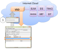
Figure 1. SHOW_SYNOP allows searching the VSO from within SSW IDL for solar data (Step 1).
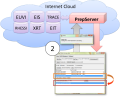
Figure 2. Data found with SHOW_SYNOP can be sent to the PrepServer for pre-processing (Step 2).
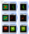
Figure 3. This figure shows examples of image data displayed with PLOTMAN. The images in the first two columns show pre-processed images. The third column shows the images in column one overlaid as contours on the images in column two (Step 3).


Minimum Requirements
- IDL 6.4
- Sun Java 1.5
- SolarSoftware (SSW) with GEN package (standard)
SHOW_SYNOP IDL Widget
Step 1: Finding the Data
SHOW_SYNOP shown in Figure 4 is an IDL graphical user interface (GUI) to search for and retrieve instrument data within a specified time interval using the VSO or other data finding facilities.
Search results can be directly downloaded into the active SSW IDL environment. To start searching with SHOW_SYNOP, first open the GUI by typing SHOW_SYNOP in your SSW IDL environment command-line. The red box highlights the VSO search form with "Start Time" and "End Time" specifying the search interval and "remote sites ->" defining the instrument (TRACE in this example). Click on the "Search" button to query the VSO for data files that will be displayed in the list below the search form shown in the green box in Figure 5.
For information on command-line VSO data searching, please click here
- SHOW_SYNOP for finding data
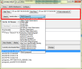
Figure 4. This is a screen shot of the SHOW_SYNOP GUI used to find and retrieve specific data sets within a given time interval. The red box indicates the VSO search form (start/ent time and instrument). This screen shot also shows the extensive list of instruments available for search.
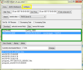
Figure 5. The green box marks the result list window in SHOW_SYNOP, and the yellow-framed button opens the configuration menu.


Step 2: Pre-processing
Typically, instrument data found with the VSO are unprocessed level-0 data. The PrepServer offers remote pre-processing of those data from within SHOW_SYNOP or from the IDL command-line before or after downloading. In SHOW_SYNOP, search results are displayed in the list underneath the VSO search form (see Figure 5, green box). There are two different pre-processing behaviors configurable:
- By default a click on "Download" retrieves the level-0 data file, stores it on the local hard drive and adds it to a list (Figure 6, blue box). The level-0 data file is pre-processed by selecting it in the blue box and clicking on "Display". This uploads the level-0 data file to the PrepServer where it is pre-processed, and downloads the pre-processed product to the local hard drive.
- In auto-preprocessing mode, which can be activated in the configuration menu (Figures 5 and 7, yellow box), SHOW_SYNOP sends the URL of the level-0 data file to the PrepServer and only downloads the pre-processed data.
In case of zipped data files (e.g. TRACE), SHOW_SYNOP opens a selection widget to help choosing the desired image(s) (see Figure 8).
Please note: SHOW_SYNOP and the PrepServer are dependent on data providers for downloading speed. Be aware that downloading data may take a few minutes, during which SHOW_SYNOP or your SSW IDL session may be unresponsive.
For information on command-line data pre-processing, please click here
- SHOW_SYNOP for downloading and pre-processing data
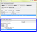
Figure 6. In this screen shot of SHOW_SYNOP the window highlighted in blue indicates the local file repository with level-0 and pre-processed data files.
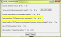
Figure 7. This options menu allows configuring the pre-processing behavior: download level-0 data or request pre-processed data.
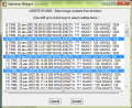
Figure 8. When pre-processing a TRACE data file that contains multiple TRACE images, a selection widget will open allowing picking a set of images.


Step 3: Visualizing
The data are visualized with PLOTMAN, which handles different data types such as light curves, images, spectra, and spectrograms. It provides basic display operations such as zooming, image overlays, solar rotation, etc. To display data with PLOTMAN from within SHOW_SYNOP, simply select a data file (Figure 6, blue box) and click on "Display". If the data file has already been pre-processed, it will be displayed immediately in a PLOTMAN window. Otherwise, it is first sent to the PrepServer for processing. If multiple files have been selected, all are displayed in the same PLOTMAN window (see Figures 9, 10, and 11).
Like all other GUIs discussed in this nugget, PLOTMAN can also be called from the command-line. Examples can be found here.
- Example images displayed with PLOTMAN

Figure 9. This figure shows PLOTMAN displaying an XRT image (January 25 2007 06:56:56) that has been pre-processed with default settings by the PrepServer
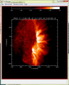
Figure 10. This figure shows PLOTMAN displaying a TRACE image (171 A, January 25 2007, 06:15:09) that has been pre-processed with default settings by the PrepServer. If multiple images were selected in the selection window (see Figure 8), they can be accessed by clicking on "Window_Control" in PLOTMAN's menu panel at the top.
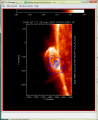
Figure 11. This figure shows PLOTMAN displaying an contour overlay of a reconstructed RHESSI clean 6-12keV image on an EIT image (171 A, January 25 2007, 07:00:13). The reconstruction of the RHESSI image as well as the pre-processing of the EIT images was done with the PrepServer.


IDL Command-Line Tools
Step 1: Finding the Data
The VSO search can be initiated directly from the IDL command-line using the procedure VSO_FILES. Two different search strategies are supported:
- An interval search that returns URLs to files containing data for the specified interval.
- A proximity search that returns a URL to the data file that is closest to the specified time.
Data for the following instruments can be searched:
- euvi
- eit
- xrt
- eis
- trace
- aia
VSO_FILES does not download any data files. Instead, SOCK_COPY or VSO_PREP (see next section) are used.
Step 2: Pre-processing
VSO_PREP allows for data pre-processing from an IDL command-line without the requirement of a local installation of instrument software or calibration data. VSO_PREP takes as a minimum a local file or a URL to a remote file for a parameter. If a URL is provided then the PrepServer will download the data and send them back pre-processed; otherwise they are uploaded to the PrepServer, pre-processed, and downloaded.
The following instrument data can be pre-processed:
- euvi
- eit
- xrt
- eis
- trace (single and zipped files)
- rhessi (image reconstruction)
Step 3: Visualizing
PLOTMAN displays level-0 and pre-processed data. It is integrated with VSO_PREP and allows visualizing data returned by VSO_PREP with one command.
Examples
- All examples demonstrate steps 1-2-3 on the command-line with the tools described above
- All examples can be copy-pasted into IDL and run from the command-line
Example 1
; Step 1: Search the VSO and return a URL to the XRT image closest to January 25 2007 06:57
; Step 2: Pre-process that data file and create an XRT object (xrt_obj)
; Step 3: Display the data file with PLOTMAN using standard coloring (see Figure 9)

xrt_file = [f]vso_files[/f]('25-Jan-2007 06:57', instr='xrt')
[p]vso_prep[/p], xrt_file, oprep=xrt_obj
xrt_obj->[p]plotman[/p], /colors
Example 2
; Step 1: Search the VSO and return URLs to EIT images that have been observed between January 25 2007 06:45 and January 25 20007 07:15
; Step 2: Pre-process one EIT image at the time and...
; Step 3: ...display it with PLOTMAN using standard coloring. All images are displayed in the same PLOTMAN window.

eit_files = [f]vso_files[/f]('25-Jan-2007 06:45', '25-Jan-2007 07:15', instr='eit')
FOR i=0, N_ELEMENTS(eit_files)-1 DO BEGIN $
 [p]vso_prep[/p], eit_files[i], oprep=eit_obj & $
 eit_obj->[p]plotman[/p], /colors, plotman=p & $
ENDFOR
Example 3
; Step 1: Search the VSO and return a URL to the TRACE data file closest to January 25 2007 07:00
; Step 2: The TRACE data file contains multiple images. Pre-process images one to 5 and create TRACE objects for them (trace_obj).
;         Not specifying an index would result in VSO_PREP opening the selection widget as shown in Figure 8.
; Step 3: Display all TRACE images in PLOTMAN using standard coloring '''(see Figure XXX)'''

trace_file = [f]vso_files[/f]('25-Jan-2007 07:00', instr='trace')
[p]vso_prep[/p], trace_file, image_no=[1,2,3,4,5], oprep=trace_obj
trace_obj->[p]plotman[/p], /colors
Example 4
; Step 1: Not required
; Step 2: Use VSO_PREP to reconstruct a RHESSI clean 6-12keV image on the PrepServer
; Step 3: Display RHESSI image with PLOTMAN using standard coloring '''(see Figure XXX)'''

[p]vso_prep[/p], instrument='rhessi', im_time_interval=['25-Jan-2007 06:53:44', '25-Jan-2007 06:57:40'], image_alg='clean', im_energy_binning=[6,12], oprep=rhessi_obj
rhessi_obj->[p]plotman[/p], /colors
Example 5
; Step 1: Search the VSO and return a URL to the EUVI data file closest to January 25 2007 06:57
; Step 2: The EUVI image is pre-processed (incl. rolling) and an EUVI object is created (euvi_obj)
; Step 3: Display the EUVI image in PLOTMAN using standard coloring '''(see Figure XXX)'''

euvi_file = [f]vso_files[/f]('25-Jan-2007 06:57', instr='euvi')
[p]vso_prep[/p], euvi_file, /roll, oprep=euvi_obj
euvi_obj->[p]plotman[/p], /colors
Conclusion
Documentation
Contacts
- SHOW_SYNOP: Dominic Zarro (dominic dot zarro at nasa dot gov)
- PrepServer: Laszlo I. Etesi (laszlo dot etesi at nasa dot gov)
- PLOTMAN: Kim Tolbert (kim dot tolbert at nasa dot gov)