Weekly Report 29Apr2011: Difference between revisions
imported>Agopie |
imported>Agopie |
||
| Line 18: | Line 18: | ||
The plots below are summarized at | The plots below are summarized at the end of the series of plots. | ||
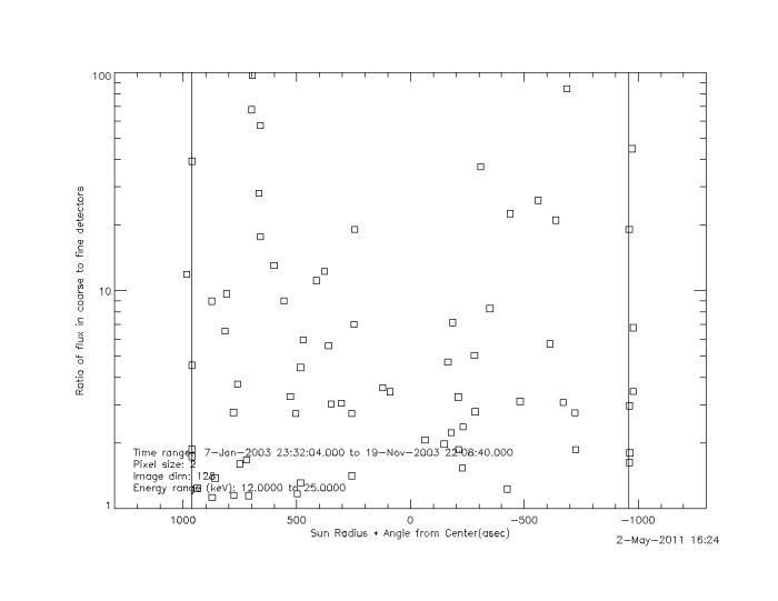
[[File:Ratio coarse fine.jpg|center|thumb|700px|The ratio of the flux from the images using detectors 6 to 9 divided by detectors 1 to 5.]] | [[File:Ratio coarse fine.jpg|center|thumb|700px|The ratio of the flux from the images using detectors 6 to 9 divided by detectors 1 to 5.]] | ||
| Line 37: | Line 37: | ||
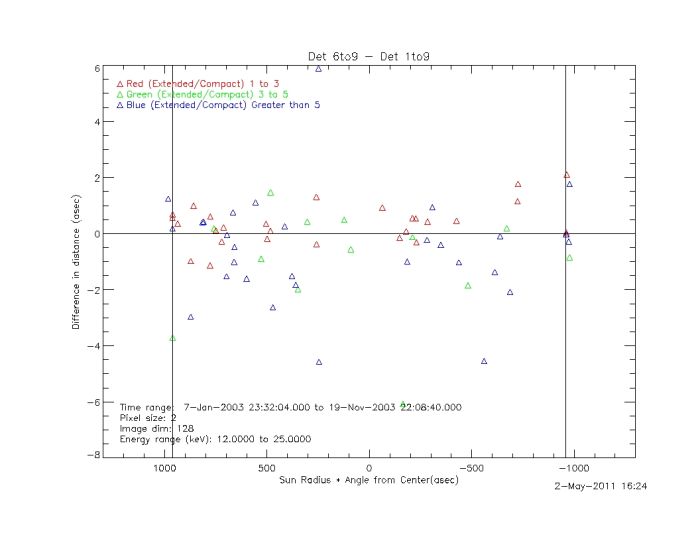
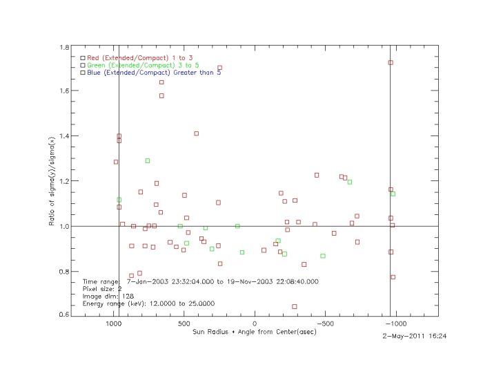
[[File:Ratio coarse.jpg|center|thumb|700px|The ratio of the standard deviation in the y direction over the standard deviation in the x direction for an image made with detectors 6 to 9.]] | [[File:Ratio coarse.jpg|center|thumb|700px|The ratio of the standard deviation in the y direction over the standard deviation in the x direction for an image made with detectors 6 to 9.]] | ||
The plots above show | |||
Revision as of 06:04, 3 May 2011
RHESSI Albedo Image Test
RHESSI Clean Imaging techniques were used to image a large number of flares. For each flare three different detector combinations and two different energy bands were used. The following parameters were used: The flares used were decided upon by the RHESSI response in the 25keV-50keV bands.
- Time: Decided by the peak of the 25keV-50keV energy band for each flare
- Energy: 12keV to 25keV, or 25keV to 50keV
- Detectors: 1 to 9, or 1 to 5,or 6 to 9
- Pixel Size: 2 arcsec by 2 arcsec
- Image Size: 128 pixels by 128 pixels
- Clean Beam Width Factor = 2
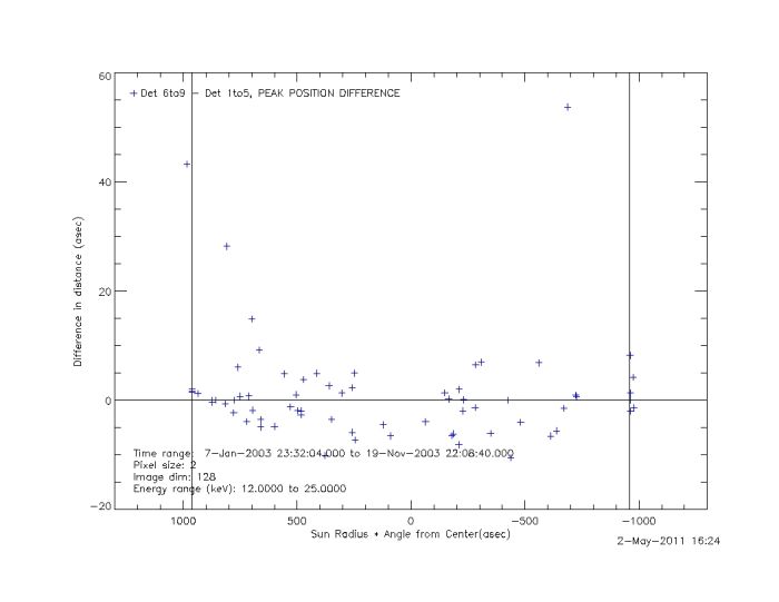
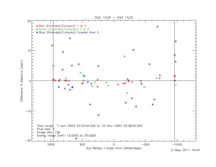
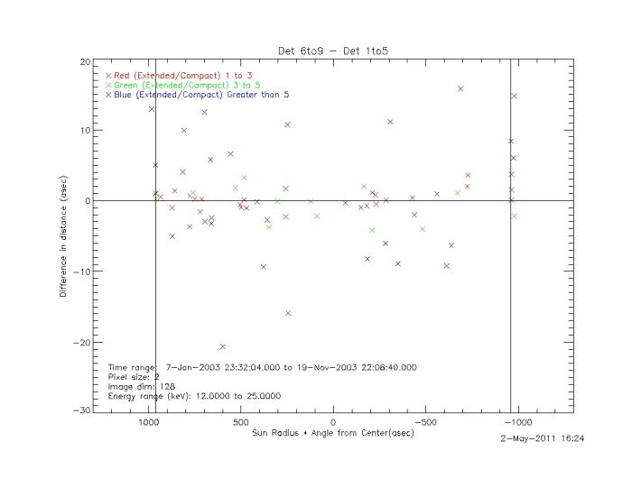
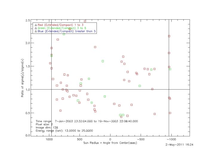
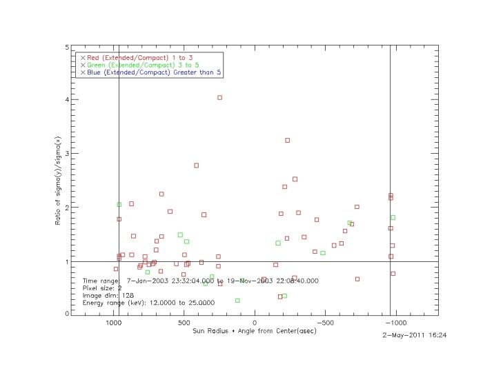
Clean images were made with each for each energy band with each detector combination. For each image the centroid of the source was measured, the total flux in the image was measured, and the standard deviation in the x and y direction for each source was measured. Using these measurements the plots below were made.
The plots were adjusted for the change in solar radius as observed from the earth at the time of the flare. All plots as a function of distance were made with an x axis as a ratio of the distance to limb at the time. An average value of 960 arcsec was added to the ratios for scaling purposes.
The plot below shows the distance to the limb in arcsec as a function of time.
The plots below are summarized at the end of the series of plots.
The plots above show

