Blind Image Analysis

Images Reconstructed by Brian Dennis

Images were reconstructed using Clean and pixon for the first four test cases using the following instructions from Richard Schwartz:

Instructions

Here is the link to the download with the files needed to run your blind image reconstructions http://hesperia.gsfc.nasa.gov/~richard/blindtest.zip Download it and unpack it into a directory. There are a few minor changes in files that will go online next week. I didn't want to chance breaking everything over the weekend by putting this all in SSW.

Get into sswidl in the directory where you unpacked these files. Use an empty one or not as you please.

From the command line

 .run blind_image_analysis_prep

This builds your image object, obj, and loads in the simulated calib_eventlist (stacked) of your choice. The file is set to use image 0 right now but if you look in the file you can see how to load in the other three as you choose. Once you use the oc->newdata method you can't go back to acquiring data normally in that image object without doing this oc->newdata, /clear

Note that this is the calib_eventlist object, OC, one of the constituents of the image object, OBJ

Also, using the seed causes the poisson deviates to be used for the simulation. If you set seed to a fixed value, use a number gt 100, then you'll get the same values every time. Calling it without using seed will send in the expected values for the counts without any poisson simulation.

You can use this OBJ for all of the images without regeneration, and for any and all analysis routines.

To use Image I

 oc->setnewdata, pcbe[*,I],seed=seed

These next two lines will cause the current image analysis routine to use the new data set

 obj-> set, det_index_mask= [0B, 1B, 1B, 1B, 1B, 1B, 1B, 1B, 1B]
 obj-> set, det_index_mask= [1B, 1B, 1B, 1B, 1B, 1B, 1B, 1B, 1B]

I will make some changes next week so send in your requests. I will also make some new files of calib_eventlists from other images of my choosing. These were designed by John Brown. That is a big hint.

Richard Schwartz richard.schwartz@nasa.gov

Test Image #1 (i = 0)

These pixon and Clean images show that there are two main sources with the north-east source appearing loop shaped. The pixon image shows an extended elliptical source surrounding the two main compact sources. The Pixon Modulation Profiles show that there are acceptable values of the C-statistic for all detectors except possibly for detector #8 where C = 2.06.

• 

  Figure 1(a). Pixon image with overlaid Clean image white contours. Clean image made with natural weighting, 128 x 0.3 x 0.3 arcsecond pixels, and clean_beam_width_factor = 2.0.

• 

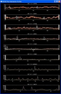
  Figure 1(b). Pixon Modulation Profiles.

Figure 1 (sam) TOP: clean images (uniform weighting) with different subcollimator combinations (s1-9, s2-9, s3-9). TOP MIDDLE: same for natural weighting. BOTTOM MIDDLE: MEM_NJIT images for different subcollimator combinations. BOTTOM: UV smooth (s 3-9)

Figure 1 (anna) uv_smooth images with different subcollimator combinations (s1-9, s2-9, s3-9).

Test Image #2 (i = 1)

This test image appears as a line source, perhaps a series of up to four compact sources, with a separate weaker source to the south-west. Pixon shows an additional extended almost circular source surrounding these compact sources. The Pixon Modulation Profiles show surprisingly large values for the C-statistic with numbers over 4.0 for all detectors except detector #7 where C = 3.45.

Figure 3. Pixon image with overlaid white contours of Clean image. The Pixon image was made with all defaults except a pixon_sensitivity of 0.5. The Clean image was made with 128 x 0.3 x 0.3 arcsecond pixels using natural weighting and a clean_beam_width_factor of 2.0.

Figure 2 (sam) TOP: clean images (uniform weighting) with different subcollimator combinations (s1-9, s2-9, s3-9). TOP MIDDLE: same for natural weighting. BOTTOM MIDDLE: MEM_NJIT images for different subcollimator combinations (s1-9 did not converge). BOTTOM: UV smooth (s 3-9)

Figure 2 (anna) uv_smooth images with different subcollimator combinations (s1-9, s2-9, s3-9).

Test Image #3 (i = 2)

This Clean image showing just the Clean components suggests that there is significant fine structure in this source but the details probably can't be trusted. The details do not shown up with Pixon, partly because Pixon cannot be used with pixels smaller than 1 arcsecond square.

Figure 3 Image shows a Clean image in color with the pixon image overlaid as white contours. The Clean image was made with uniform weighting,a gain of 0.01, 1000 iterations, and a beam width factor of 10. The latter factor allows the individual Clean components to be shown. The Pixon image was made with 1 arcsecond pixels using all nine detectors.

Figure 3 (sam) TOP: clean images (uniform weighting) with different subcollimator combinations (s1-9, s2-9, s3-9). TOP MIDDLE: same for natural weighting. BOTTOM MIDDLE: MEM_NJIT images for different subcollimator combinations. BOTTOM: UV smooth (s 3-9)

Figure 3 (anna) uv_smooth images with different subcollimator combinations (s1-9, s2-9, s3-9).

Test Image #4 (i = 3)

Figure 4 Pixon image with Clean image overlaid as white contours. Clean image was made with uniform weighting, a gain of 0.05, 500 iterations,a Clean Beam Width Factor of 2.0, and 64x64 0.5 arcsecond pixels.

Figure 4 (sam) TOP: clean images (uniform weighting) with different subcollimator combinations (s1-9, s2-9, s3-9). TOP MIDDLE: same for natural weighting. BOTTOM MIDDLE: MEM_NJIT images for different subcollimator combinations. BOTTOM: UV smooth (s 3-9)

Figure 4 (anna) uv_smooth images with different subcollimator combinations (s1-9, s2-9, s3-9).